无双梦溪石(无双梦溪石最新番外)
有,可以点我头象点我头象,。…了解一下无双
中国古典文学在浩如烟海的中国古典文化宝库中,文言文作为中华民族悠久历史与深厚文化的瑰宝,承载着丰富的思想、情感与哲理。收藏这些古代经典的文言文佳作,不仅可以丰富个人的文化底蕴,还能极大提升语言理解和鉴...
小说:饭局上,美女大佬备受追捧,却假装跟前夫没关系乔紫萱向桌上众人介绍道:“这位是周安娜,我的救命恩人,珠宝设计师,旁边这位是......”余佳一接上:“何琳,我们工作室的大美女。”大家点头示意。姜明...
师父?师夫!顶好看的 推荐如下:《报告!帝君你有毒!》(由翎夭夭创作,小说的主角是凌止昔萧寒。)《师叔祖,放过咸鱼吧!》(由欲归晚创作,小说的主角是沐云舒玄御。)《嫁给帝尊后我掉马了》(由初雪妖娆创作...
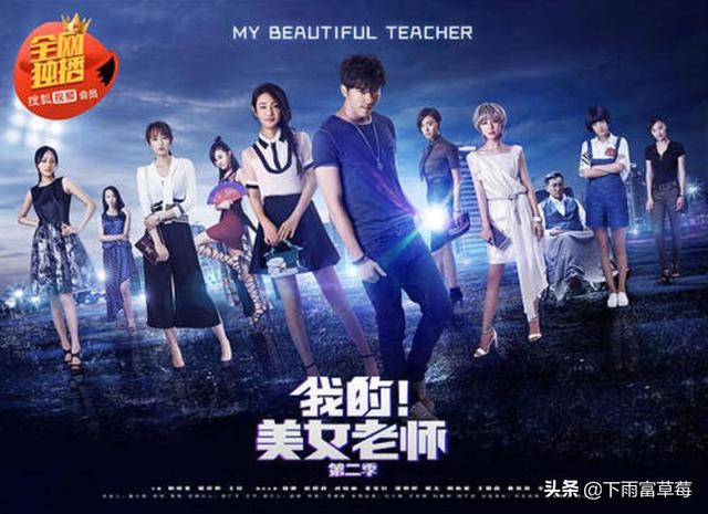
苏姬是由网络作家黑夜de白羊创作的小说《我的美女老师》中的女主角。秦朝的正牌女友。苏南市苏家三小姐,黑暗教廷女皇。原系嵩山宝台寺外门弟子,意外变为吸血鬼后成为黑暗教廷教皇,被秦朝炼成天皇魔傀,为安晴倍...
异能高手,校花的贴身高手,很纯很暧昧《丧末时代》这个书不错,没有一点异能,而且是行尸走肉那种多线人物发展!起点上的,作者说是前300万字免费! 超级电能,最终智能,重生之都市天骄,这三本一个作者,还可...
她最后成了皇贵妃,和四爷幸福美满的生活下去,子孙满堂。《四爷的心尖宠妃》是一部古代言情类型网络小说,作者是雪中回眸,目前已完结,共计1508章。...